Stress-Based Timeslice Design
Intelligent temporal modeling through operational stress identification
VerveStacks transforms the 8760-hour modeling challenge into intelligent timeslice structures by identifying periods of maximum operational stress in high-renewable energy systems. Each ISO receives its own unique timeslice definition, tailored to that country's specific demand patterns, renewable resource characteristics, and operational challenges. Rather than using fixed temporal patterns, we construct hypothetical "clean" energy scenarios for each ISO and analyze when storage, ramping, and dispatchable resources face their greatest challenges.
Spain: Mediterranean solar patterns |
Brazil: Tropical hydro-wind diversity |
Spain: Solar-driven daily peaks |
Brazil: Seasonal hydro variations |
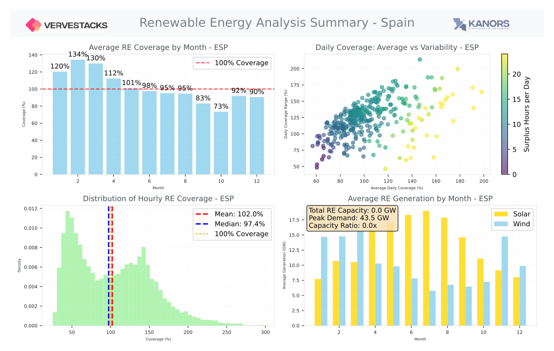
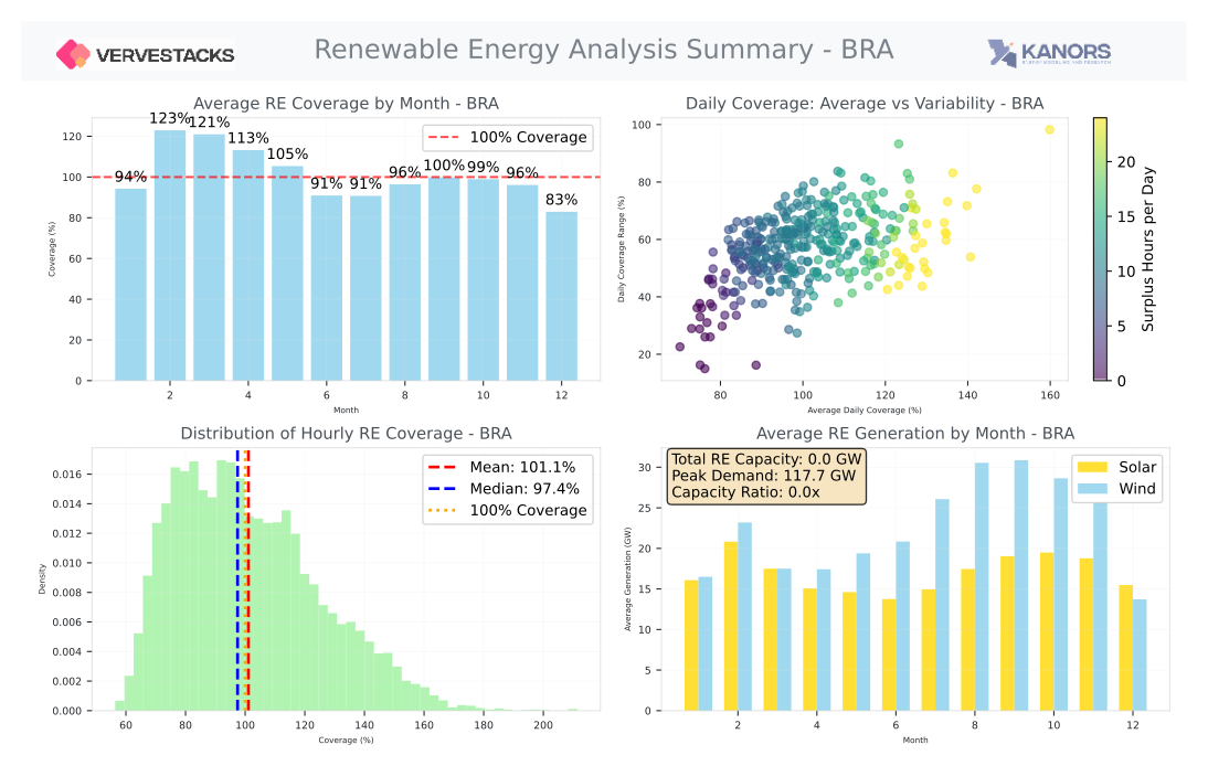
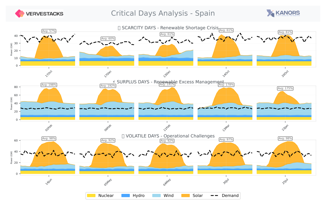
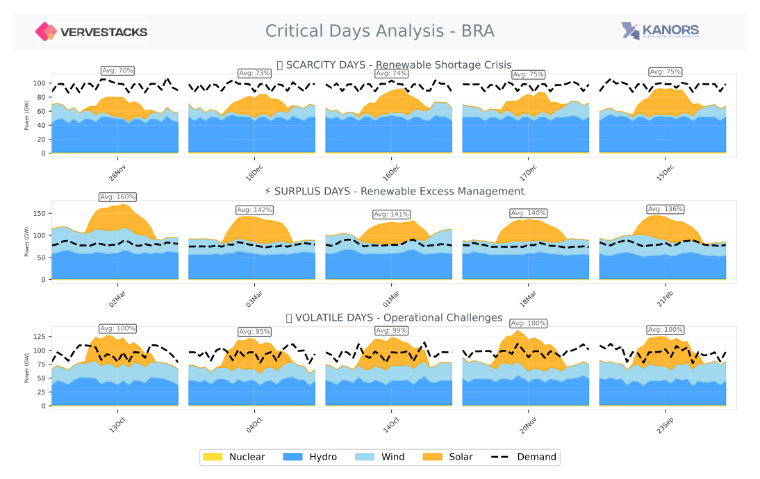
What the four charts show
Spain and Brazil both have clean supply that covers about 100% of demand on average over the year. The method shows that the averages hide opposite problems.
- Spain's stress is daily. Hourly coverage is split in two: a peak near 50% (nights) and another near 140% (sunny middays). The surplus days (late winter, wind plus sun at 175–198% of demand) and the scarcity days (October and December, 57–61%) are a season apart, and in summer the volatile days swing from about 15 GW at night to 55 GW at noon against flat demand. A model of Spain needs hourly detail inside the day, where batteries and flexible plant earn their keep.
- Brazil's stress is seasonal. Hydro gives a steady base of 45–55 GW every day, so hourly coverage has a single peak and a narrow spread. The scarce days sit together in late November and December (70–75%), and the surplus days in the February–March wet season (136–160%). A model of Brazil needs to get the seasons right; daily swings matter less.
- The same method, different time slices. Neither result was set by hand. Each comes from running the same four stages on each country's own data, which is why every country gets its own time-slice definition.
The charts were made with an earlier pipeline version. The bottom-right panel's "Total RE capacity: 0.0 GW" label is a display fault in that version, not a property of the model.
Status in the current model library
The stress-day selection described in Stages 3 and 4 is implemented and can be switched on per country. The options shipped in today's library builds (ts_012 to ts_288, and the dry- and wet-year ts_072P10 and ts_072P90) use the day-based seasonal clustering of Stage 4 on its own: the 365 days are grouped into 4 to 24 seasons by net-load similarity, and the hours into 3 to 12 periods of the day. Stress-day options are added as rows in the configuration sheet described below.
Methodology Overview
The stress-based approach follows a systematic four-stage process applied individually to each ISO:
- National Shape Aggregation: Transform grid-cell renewable profiles into realistic national patterns
- Clean Supply Construction: Build hypothetical zero-emission supply scenarios using existing assets plus renewables
- Stress Period Identification: Analyze supply-demand mismatches to rank operational challenges
- Intelligent Aggregation: Select critical periods for hourly modeling, cluster the remainder
Every ISO gets its own analysis: A country with abundant hydro will have different stress periods than one dominated by solar potential. Arctic countries face different seasonal challenges than tropical ones. The methodology adapts to each country's unique energy landscape.
The goal is not energy balance, but stress identification—finding the days and weeks that will test each country's grid flexibility most severely.
Stage 1: National Renewable Shape Aggregation
From Grid Cells to National Patterns (Per ISO)
Individual renewable energy grid cells often exhibit unrealistic characteristics—including complete zero-generation periods that would never occur in diversified national portfolios. For each ISO separately, we address this through economic aggregation:
- Demand-Constrained Selection
-
Using actual national electricity generation as the target, we select only the most cost-effective grid cells rather than theoretical maximum potential.
- Economic Ranking
-
Grid cells are sorted by levelized cost of energy (LCOE), ensuring deployment follows economic logic rather than resource abundance alone.
- Spatial Portfolio Effect
-
Capacity-weighted averaging across selected grid cells eliminates unrealistic zero-generation periods while preserving temporal variability needed for stress analysis.
Result: Realistic national renewable profiles that reflect actual deployment economics and geographic diversity, suitable for operational stress analysis.
Stage 2: Clean Supply Construction
Building the Hypothetical Zero-Emission Scenario (Per ISO)
For each country individually, we construct a complete 8760-hour "clean" electricity supply using a systematic approach:
- Baseline Generation Foundation
-
- Nuclear: Existing capacity operating as flat baseload throughout the year
- Hydro: Existing capacity shaped to follow monthly supply patterns from EMBER data - shaped to follow demand patterns within each month
- Renewable Gap-Filling
-
- Calculate residual electricity demand after accounting for nuclear and hydro
- Fill this residual with solar and wind capacity using economic logic and realistic technology shares
- Apply national renewable shapes derived from grid-cell aggregation
- Technology Portfolio Logic
-
Solar and wind shares are determined through enhanced LCOE calculations combined with historical deployment patterns, preventing unrealistic technology monopolization while maintaining cost-effectiveness.
Result: Complete 8760-hour supply profile representing a realistic zero-emission electricity system for stress testing.
The two stages that pick the time slices, as one picture:
Surplus: highest daily average.
Volatile: highest variance, among days averaging 100% or less. No day is picked twice.
s5p5v5_d. Weekly selection currently takes the scarcest weeks only.Each time-slice option is a row in the stress_periods_config sheet of VS_mappings.xlsx. A row sets the number of seasons and of daily periods, the hydro year, and optionally how many scarcity, surplus and volatile days (or scarcity weeks) to keep hour by hour. Stress options are named by the selection: s scarcity, p surplus, v volatile, then _d for days or _w for weeks, so s5p5v5_d keeps the top five days of each list and s2_w the two scarcest weeks. Clustering-only options are named by their slice count, as in ts_048.
Stage 3: Stress Period Identification
Coverage Analysis Framework
The heart of the methodology lies in coverage analysis—comparing clean supply to electricity demand hour by hour:
Coverage Ratio = (Clean Generation) / (Electricity Demand) × 100%
Three Stress Categories
- Scarcity Periods (Coverage < 100%)
-
Hours when clean generation falls short of demand, requiring storage discharge, imports, or dispatchable backup. These periods test the adequacy of storage capacity and flexible resources.
- Surplus Periods (Coverage > 100%)
-
Hours when clean generation exceeds demand, requiring storage charging, exports, or curtailment. These periods test grid absorption capacity and storage charging infrastructure.
- Volatile Periods (High Coverage Variability)
-
Hours with rapid coverage changes, requiring maximum ramping capability and operational flexibility. These periods test the speed and agility of grid response systems.
Operational Stress Ranking
- Days and weeks are ranked within each category, in this order, and a day picked for one list is not offered to the next:
-
- Scarcity ranking: Days with the lowest average coverage (most severe shortfalls)
- Surplus ranking: Days with the highest average coverage (most severe oversupply)
- Volatility ranking: Days with the highest variance of hourly coverage, among days whose average coverage is 100% or less (large swings on days that are already short)
Result: Three ranked lists identifying the most operationally challenging periods in each stress category.
Stage 4: Intelligent Temporal Aggregation
Configurable Critical Period Selection
From the ranked stress lists, we select varying numbers of days and weeks for explicit hourly modeling:
- Daily Stress Configurations
-
- Select top-ranked days from each category (e.g., 3 scarcity + 3 surplus + 3 volatility days)
- Each selected day retains full 24-hour resolution for detailed operational analysis
- Weekly Stress Configurations
-
- Select sustained stress weeks for extended storage and ramping analysis
- Capture multi-day operational challenges that daily analysis might miss
- Day-Based Seasonal Clustering
-
Unlike traditional month-based aggregation, VerveStacks clusters all 365 days directly into seasons based on their net load patterns. This approach captures multi-day events (such as wind droughts or sustained low-solar periods) that may span across month boundaries.
The clustering algorithm:
- Analyzes each day's net load profile (mean, peak, minimum, variability, daytime/evening patterns)
- Groups days with similar characteristics into contiguous seasons
- Enforces a minimum days-per-season threshold (default: 5 days) to prevent fragmented single-day seasons
- Preserves temporal continuity so adjacent days remain in the same cluster when patterns are similar
This day-level granularity is essential for capturing the operational reality of battery storage systems that operate on daily charge/discharge cycles, and for identifying sustained renewable droughts that stress system flexibility over multiple consecutive days.
- Adaptive Timeslice Assembly (ISO-Specific)
-
The final timeslice structure combines:
- High-resolution critical periods (hourly detail where it matters most)
- Day-clustered seasons (365 days grouped into 4-12 seasons based on net load similarity)
- Hour-clustered periods (24 hours grouped into 3-8 diurnal periods)
- Proper weighting to preserve annual energy balance
Each ISO receives its own complete timeslice definition—including both the stress periods and the day-based aggregated clusters. Germany's winter scarcity periods will differ completely from Brazil's dry season challenges or Japan's summer peak stress.
Validation and Visualization
- Stress Period Representativeness
-
Selected periods are validated to ensure they capture the full spectrum of operational challenges, from sustained shortfalls to rapid ramping events.
- Energy Balance Preservation
-
Despite focusing on stress periods, the complete timeslice structure maintains annual energy conservation and realistic operational constraints.
- Visual Diagnostics
-
Coverage analysis produces intuitive visualizations showing when and how severely the electricity system will be stressed, enabling stakeholders to understand operational challenges at a glance.
Methodology in Action: USA Case Study
The following visualizations demonstrate the stress-based methodology applied to the United States, showing how coverage analysis identifies critical operational periods.
Coverage Analysis Overview
 { width="100%" }
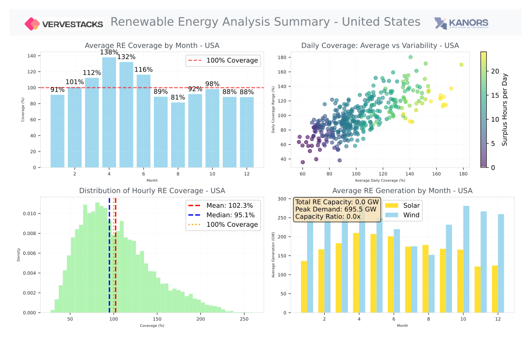
Coverage Metric Demonstration: This chart shows the complete coverage analysis for the USA, illustrating how clean generation (nuclear + hydro + renewables) compares to electricity demand throughout the year. The coverage ratio reveals when the system faces scarcity (red zones below 100%) and surplus (green zones above 100%).
Daily Stress Period Selection
 { width="100%" }
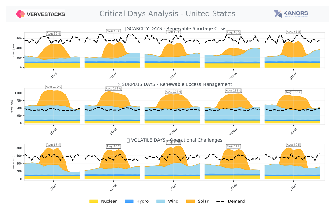
Top 5 Days from Each Stress Category: This visualization shows the selected critical days—5 scarcity days (lowest coverage), 5 surplus days (highest coverage), and 5 volatility days (highest variability). Each selected day receives full hourly resolution in the final timeslice structure.
Weekly Stress Analysis
 { width="100%" }
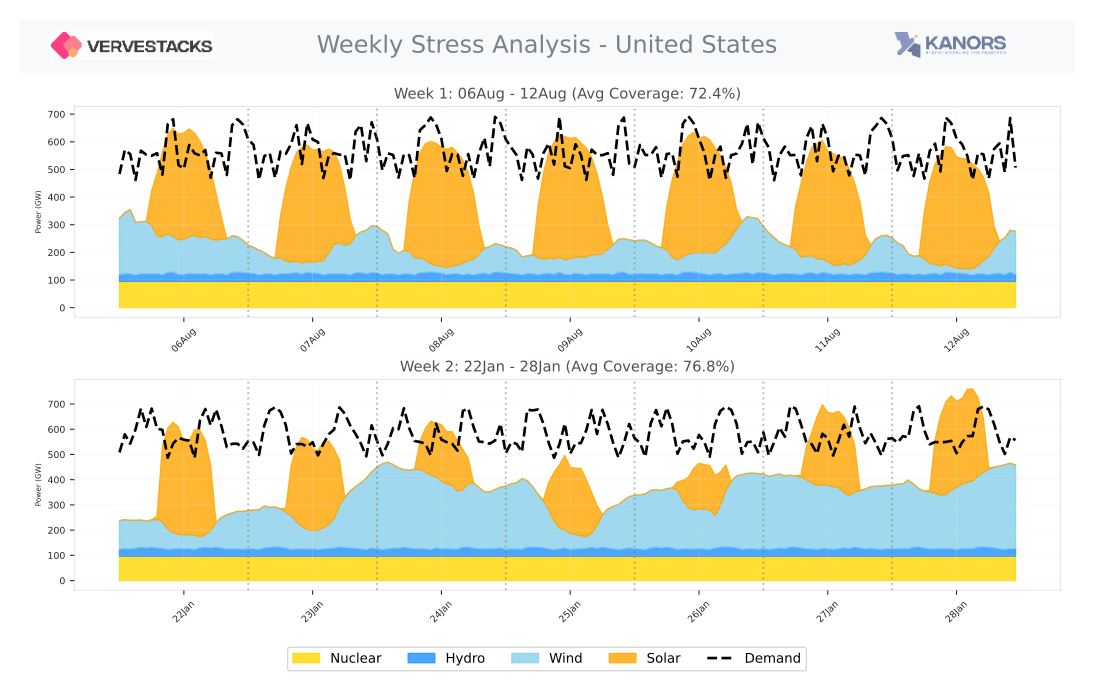
Prolonged Shortage Periods: Extended stress weeks capture sustained operational challenges that daily analysis might miss. These multi-day periods test storage capacity and sustained generation capability over longer timeframes.
Day-Based Seasonal Clustering
 { width="100%" }
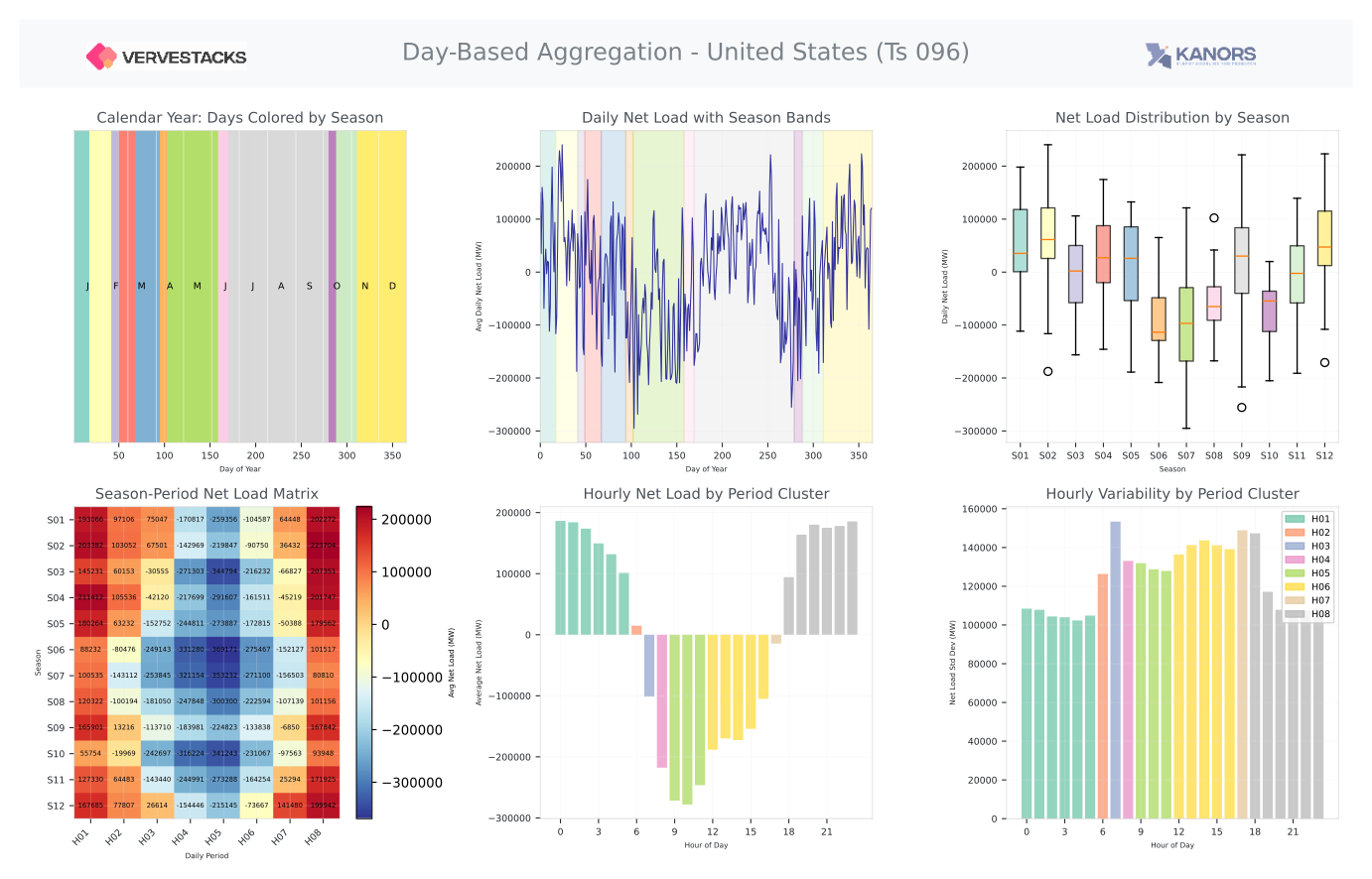
365 Days Clustered into Seasons: This visualization shows how the USA's 365 days are grouped into seasons based on net load similarity, with a calendar heatmap revealing the temporal distribution. The day-based clustering captures multi-day wind droughts and sustained low-solar periods that month-based approaches would miss. Rolling averages show how net load patterns evolve through the year, with distinct seasonal bands emerging from the clustering algorithm.
What a country model gets out of the box
The time-slice design is done for every country in the library before anyone opens the model. For each time-slice option the build writes, ready to use:
- The time-slice definition itself: which days and hours fall in which slice, with weights.
- A profile for every wind and solar cluster, each from its own weather cells, averaged into the same slices.
- Demand shapes by sector (industry, buildings, road transport) and peak factors.
- Hydro availability for the slices, including dry-year and wet-year variants (P10 and P90).
- Firmness coefficients for every wind and solar cluster, in grid models: the deepest shortfall its own hourly profile shows inside any time slice, carried into the model so averaging does not overstate what the cluster can be relied on for.
Several options ship side by side, each in its own scenario file (SuppXLS/Scen_TSParameters_<option>.xlsx); Germany's run from 12 to 220 slices. A user can check whether a result depends on temporal resolution by switching option, without rebuilding anything.
Contrasting Energy Landscapes: China Case Study
China presents a dramatically different energy landscape, demonstrating how the stress-based methodology adapts to diverse national characteristics. Where the USA shows moderate seasonal variation, China exhibits extreme contrasts between renewable abundance and scarcity periods.
China's Coverage Analysis
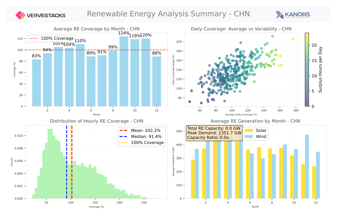 { width="100%" }
Extreme Seasonal Contrasts: China's coverage analysis reveals much sharper seasonal patterns than the USA. The massive scale of China's energy system creates distinct periods of extreme surplus (potentially over 200% coverage) and severe scarcity, reflecting the country's vast renewable resources and enormous electricity demand.
China's Daily Stress Periods
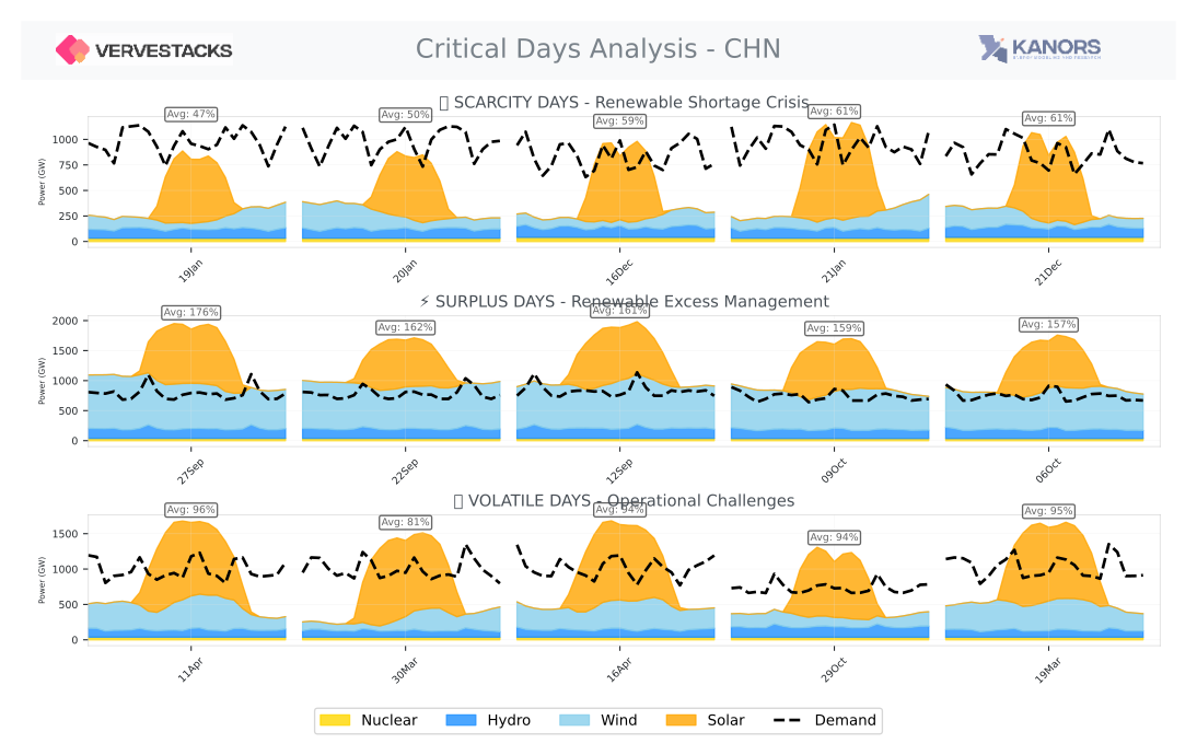 { width="100%" }
Continental-Scale Stress Patterns: China's selected stress days show the complexity of managing a continental-scale energy system. The surplus periods demonstrate the potential for massive renewable generation, while scarcity periods highlight the challenge of meeting enormous industrial and urban demand during low renewable periods.
China's Weekly Stress Analysis
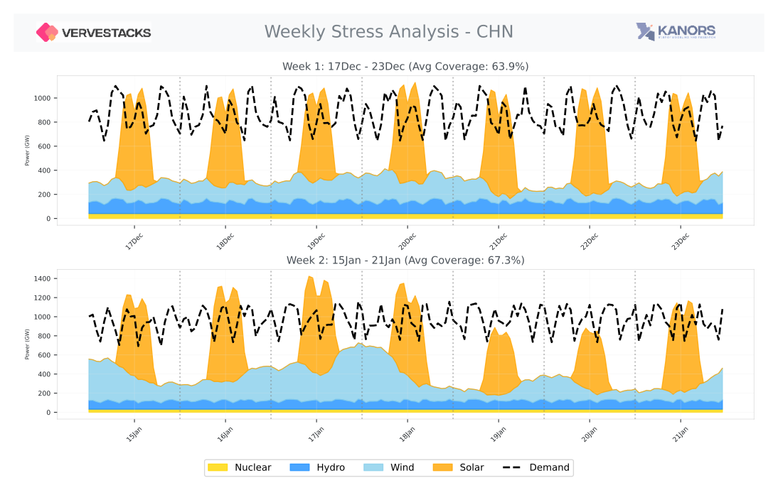 { width="100%" }
Sustained Stress at Scale: China's weekly stress periods reveal the magnitude of sustained operational challenges in the world's largest energy system. These extended periods test not just storage and ramping capability, but the coordination of resources across vast geographic distances.
China's Day-Based Seasonal Clustering
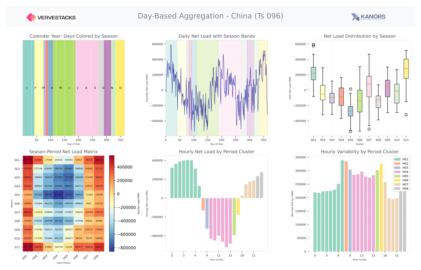 { width="100%" }
Continental-Scale Day Clustering: China's 365 days are grouped into seasons reflecting the country's vast geographic and climatic diversity. The calendar heatmap reveals how seasonal boundaries emerge from actual net load patterns rather than arbitrary calendar months. By clustering days directly, the system captures China's unique multi-day weather events, industrial demand cycles, and the interplay between northern heating demand and southern cooling loads.
Key Contrasts: USA vs China
The comparison between USA and China stress periods illustrates the methodology's adaptability:
- Scale Differences
-
- USA: Moderate seasonal variation, balanced renewable mix, regional diversity
- China: Extreme seasonal contrasts, massive scale effects, continental coordination challenges
- Stress Period Characteristics
-
- USA: Gradual transitions, moderate surplus/scarcity ranges
- China: Sharp seasonal breaks, extreme surplus potential, severe scarcity periods
- Operational Implications
-
- USA: Focus on regional balancing, moderate storage requirements
- China: Continental-scale coordination, massive storage and transmission needs
This demonstrates why every ISO requires its own unique timeslice definition—no universal template could capture both the USA's moderate seasonal patterns and China's extreme continental-scale energy dynamics.
The day-based clustering approach is particularly valuable here: a wind drought spanning late January through early February would be split across two months in traditional aggregation, but is captured as a single coherent stress event when clustering 365 days directly. This granularity matters most for countries with pronounced multi-day weather patterns that don't align with calendar boundaries.